
By now, everyone has heard or read about the terms Artificial Intelligence (AI), Machine Learning (ML) and Deep Learning. ChatGPT is currently on everyone’s lips and on social media everybody wants to show that they have also “talked” to ChatGPT. In short, the topic is currently conquering the world and it won’t be long before robots take over the world. 🤖😉
But before that happens, let’s take a look at why we can make these lovely tools in the first place. It all starts with a neural network, which is made up of many neurons. But what exactly is a neuron?
In the human body, a neuron is a cell in the nervous system that transmits signals through electrical and chemical processes. This neuron consists of a cell body, dendrites, and an axon. Dendrites receive signals from neurons, while the axon transmits signals to other neurons. Thus, neurons can be thought of as the basic building blocks of the nervous system that enable us to think, feel, and act. 🧠
In the field of artificial intelligence (AI for short), neurons are the basic elements of a neural network. In this context, a neural network builds on the idea of the human nervous system. An artificial neuron within a neural network behaves similarly to a biological neuron; it takes input signals from neurons and passes output signals to other neurons. The difference is that the inputs and outputs of artificial neurons are numerical and the weights of the connections between them are adjusted by an algorithm to learn specific tasks. Now this might sound very abstract at first, right? Let me try to illustrate this abstraction for you.
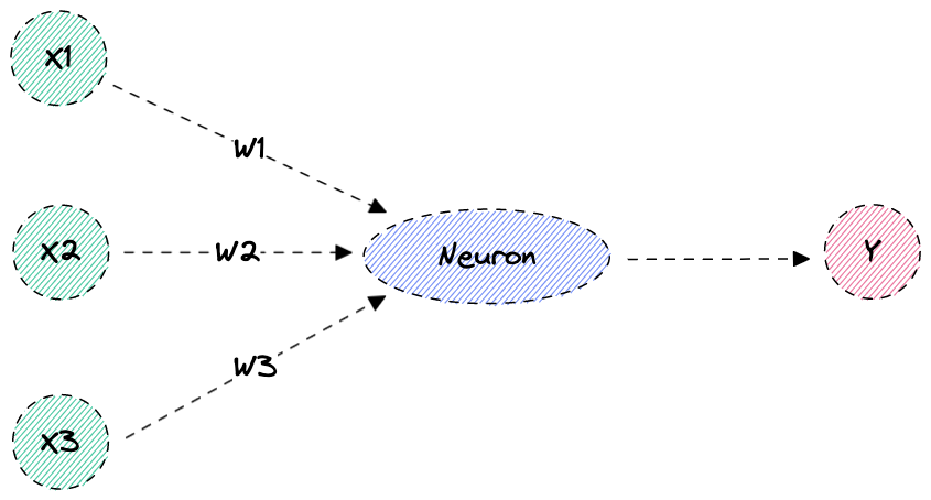
Figure: Neuron with three inputs and one output
In this picture we see how a simple neuron is constructed. The neuron has several inputs X1, X2 and X3, and an output Y. The inputs are assigned with so-called weights; the weight W1 belongs to input X1, W2 to X2 and logically W3 to X3.
The neuron now sums the inputs and the weights and passes the result to output Y, since we assume a linear activation function. We will see what an activation function is below. The formula for this calculation is as follows:
|
|
So far so good. Now let’s look at how we can make a calculation with a neuron using linear regression as an example.
Neuron using linear regression as an example
We want to look at a neuron that makes a prediction using linear regression. Here, we specify input values with the corresponding results and then calculate the prediction for an arbitrary input value on the basis of these values. Sounds complicated? Let’s shed some light on this and look at a simple example. We want to convert kilometers into miles and have the following information:
10 km –> 6.21 miles
35 km –> 21,75 miles
85 km –> 52.82 miles
Figuratively, this neuron would now look like the following. We have an input X1 with a weight of W1 and an output Y. The linear regression would for example now be calculated in our neuron.

Figure: Neuron with one input and one output
Our neuron would now have to calculate the corresponding y values using the formula for linear regression. If you don’t have the formula at hand, here it is:

Figure: Regression – Basic Statistics
Well, many probably don’t really know what to do with it now. Fortunately, there is a workaround. Python, for example, provides us with a module that allows us to easily calculate linear regression based on the values we use for prediction.
Here is one such program that performs this calculation for us:
|
|
So let’s take a closer look at the code. In lines 1 and 2, we define the points that will serve as our starting point for the prediction. It should be said here that this is not really a prediction, since there is a precise formula for converting kilometers to miles. But it serves us as a simple and illustrative example. In line 4 we import from the package scikit-learn the LinearRegression function. After that we can create a new model in line 5. We train this created model in line 6 with the already known datasets. After this is done, we can output the coefficient, i.e. the ratio, with which we get from X to Y. So we get Y now by calculating X = 250 * 0.62140936 = 155.35234.
To avoid having to do this calculation manually, Python, or scikit-learn provides us with a function that we can use to make the prediction. In line 11 we make a prediction based on the calculated coefficients and get the corresponding values.
Activation function
So now we know how a simple neuron works. However, in order to understand how a neural network works, we are still missing a crucial component, namely the activation function. An activation function is needed for a neuron to be activated or deactivated based on its inputs. In the example above, we saw that there is a linear relationship between the input and output. However, neural networks can’t really deal with linear dependencies. We will look at why this is the case very soon. What we need for a neural network is a non-linear dependency of the parameters provided to determine whether a particular neuron is activated or not. So the important thing about the activation function is that it can firstly turn a linear value into a non-linear value and that we get a value between 0 and 1 as a result. Furthermore, it still needs a defined threshold. If the output of a neuron is greater than this threshold, it is activated and the “signal” is passed on to a following neuron. Otherwise, it remains deactivated. There are several types of activation functions, such as the sigmoid function. However, we won’t further look into how exactly this function works in the context of this TechUp.
Neural Networks
Now we know how a single neuron is constructed and how an activation function works. So let’s now go one step further and take a closer look at the principle of a neural network. Neural networks are adaptive algorithms, inspired by human or animal brains, which can process input data according to complex schemes with the help of the “neurons” we have already learned about. In principle, neural networks always consist of the following four components:
- An Input Layer
- At least one Hidden Layer
- At least one activation function
- An Output Layer
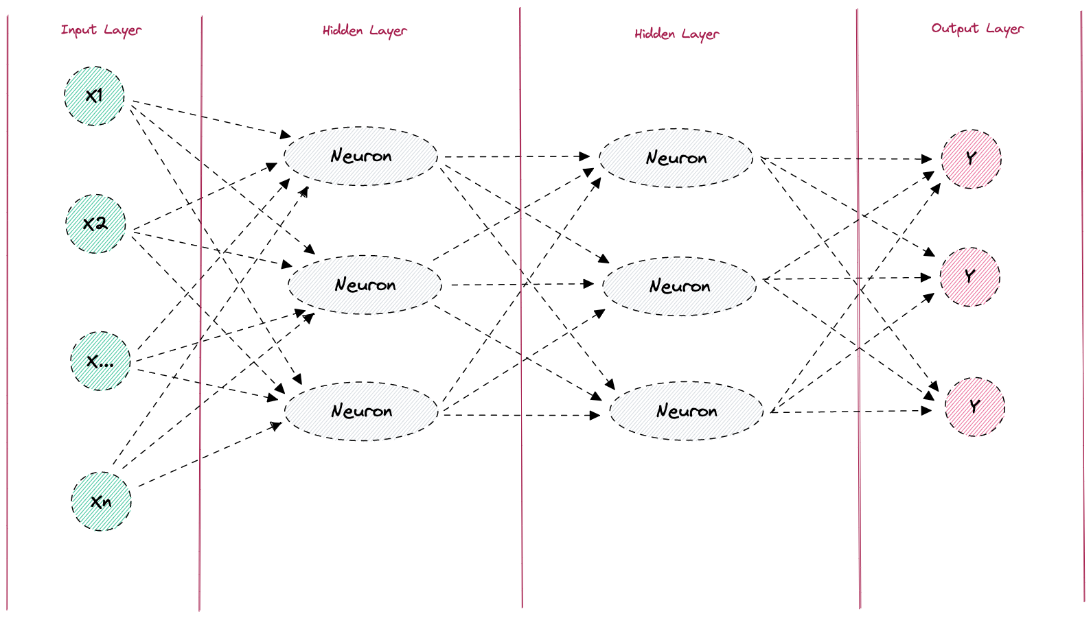
Figure: Neural Network
Let’s take a look at a practical example to see how a prediction can be made with such a neural network. A practical example would be the detection of handwritten numbers. We give the number we want to detect as input to our neural network.
In the following picture we see how a detection of the number 5 would be possible in a neural network.

Figure: Neural network for the detection of the digit 5
In the picture we see an input layer, a hidden layer and an output layer. Each neuron has an activation function, which decides whether the respective neuron is activated (also called “firing”) or whether it remains deactivated. In the Hidden Layer, the two neurons that correspond to the shapes that make up the number 5 are activated. In this case, the neuron that detects the circle remains deactivated because the threshold of 0.7 has not been exceeded. In the Output Layer, the neuron that recognizes the number 5 is then activated with the input from Hidden Layer, and the output is passed to the Output Layer. Thus, our neural network predicted that it is the number 5 with a probability of 0.9.
But what if the number had not been correctly detected? In that case, we would have to retrain our model.
Training a model
All of us have heard this before. We need to train the artificial intelligence so that we can get an accurate prediction. But what is this training all about? Let’s take a closer look at this using the number recognition in the example above.

Figure: Neural network for the detection of the digit 5 - Incorrect prediction
In the picture, we see that a 6 was accidentally detected instead of a 5. This happened because the threshold of the neuron that detects the number 6 was exceeded and the one for detecting the number 5 was not. So what do we have to do for the correct neuron to be activated next time? Well, the threshold value of the neuron for the recognition of 5 must be surpassed and the one for the recognition of 6 must be undershot. In short: We simply have to “tweak” the weighting or the threshold a little bit. The error here obviously lies within the neuron in the hidden layer, which recognizes the circle. This should not be activated, because it falsifies our result. But how can we change the weights and thresholds without manually influencing them? In a neural network this is done by means of the so-called backpropagation.
Backpropagation
In order to do backpropagation, we first need to introduce the concept of a cost function (or loss function). In machine learning models, the cost function is used to measure the error between a model’s predictions and actual outputs. The smaller the error, the better the model fits the data and the higher its accuracy. The cost function, is typically used in model optimization to adjust weights and thresholds to minimize error. This means that the cost function is essential for us to be able to train our model.
An example of a cost function could look like this. It should be said here that there are other cost functions, but we won’t look at them in this TechUp.

Figure: Neural network - cost function example
So we simply calculate the predicted value minus the real value, i.e. the value with which our model was trained. The smaller this value c is, the better our model is trained. But how can we minimize the error by finding the cost. Now we need a little bit of math again. Let’s look at the example of the simple neuron from above:
Figure: Neuron with one input and one output
As long as we train our model, the value Y (with roof) in this image is the predicted value. This means we can solve the equation as follows:
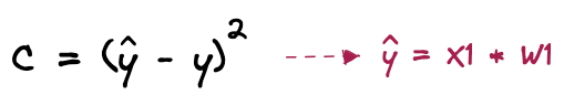
Figure: Mathematically solve cost equation - Step 1
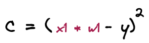
Figure: Mathematically solve cost equation - Step 2
Since Y (without roof) is always the real value, i.e. the value of the current calculation, and X1 is always a fixed input value, we see quite quickly that there is only one parameter in the above equation that we can change in order to minimize the costs, namely W1; the weight. This is exactly what happens now in backpropagation. After each training run, the cost is calculated and the weights are changed with the goal of minimizing that cost. The effort here is to bring the costs as close to zero as possible.
With this explanation I’ll conclude my TechUp today and hope I was able to give you a basic understanding of how a neuron, and based on that a neural network works. We at b-nova find this topic really exciting and will certainly continue to explore it. Stay tuned! 🔥
Here you can find another great TechUp on this topic: The Basics of AI, Machine Learning and Deep Learning. 🚀
Stefan Welsch – Pionier, Stuntman, Mentor. Als Gründer von b-nova ist Stefan immer auf der Suche nach neuen und vielversprechenden Entwicklungsfeldern. Er ist durch und durch Pragmatiker und schreibt daher auch am liebsten Beiträge die sich möglichst nahe an 'real-world' Szenarien anlehnen.