Making Complex Data Simple - Understanding Decision Trees in Machine Learning

Besides Neural Networks, using Decision Trees is another way to draw conclusions from complex data using Machine Learning. Decision trees are a type of tree structure consisting of nodes and edges. At each node, a question is asked, the answer to which determines which edge to follow further down the tree. At the end of the path is an output that represents the decision of the tree.

Figure: Example tree

Decision trees are generally divided into two categories: Classification Trees and Regression Trees. Classification trees are used, as the name suggests, to classify input data with respect to specific categories, while regression trees are used to predict numerical values.

A Classification Tree Example

An example use case for a classification tree is the differentiation of plants by their species. Characteristics such as growth size, flower color, flower shape, etc. can be used as input to make individual decisions at the nodes of the tree, e.g. based on the growth size of the plant, and finally arrive at a category, in this case the plant species.

A Regression Tree Example

A typical example of a regression tree is predicting the selling price of a house. Features such as the number of rooms, the size of the property, the location, etc. can be used in the tree to make individual decisions, and finally arrive at a price. The possible outputs are not limited to specific values, but can take any numerical value.

Algorithms

There are various algorithms to create or train decision trees. In this TechUp, we will first look at the Random Forest algorithm, and then create a decision tree using an example, as well as discuss the advantages and disadvantages of Decision Trees.

Random Forest

The Random Forest algorithm is an ensemble learning algorithm in which several decision trees are created independently of each other. To arrive at a decision from a given input, the decisions of the individual trees are combined and summarized into an output. This approach is also called Bagging (Bootstrap Aggregating).

The advantage and idea behind this approach is that the different trees can compensate for errors of the individual trees. A single tree can lead to a bad output due to random decisions or a bad input dataset. By combining several trees, this error can be compensated.

To ensure that the results of the individual trees are independent of each other and differ from each other, the trees are not all trained with the same or complete dataset. Instead, each tree is trained using a subset of the complete dataset.

When building a tree, the decision at the individual nodes is not based on all features, but on a random subset of the features. This procedure ensures that the trees differ from each other and are trained independently of each other. At the end, the results of the trees are combined into one output.

A Simple Random Forest Example

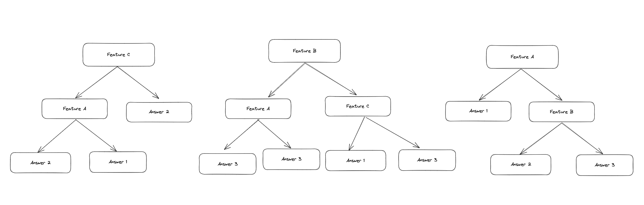
This all sounds relatively complex. However, with an example, the whole thing becomes much easier to understand: In this example, we want to classify a plant based on a dataset and decide whether it is either an apple tree or a tomato plant. The dataset consists of the features leaf size, fruit size and growth height. A total of 3 trees are created:

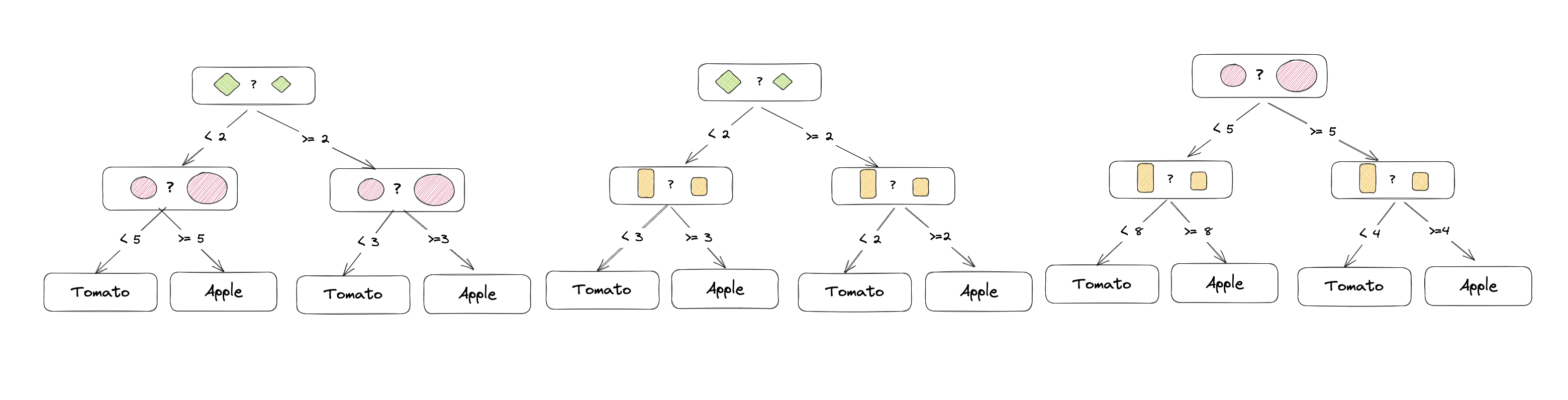
The first tree distinguishes based on leaf and fruit size, the second based on leaf and growth height, and the third based on fruit and growth height. The trees are trained independently and the results are combined. Each tree makes the decision that best fits the features.

The decisions of the first tree could look like this: If the leaf and fruit size exceed a certain size, it is an apple tree, since most data points with these values belong to an apple tree. If the values are below that, it is a tomato plant, since most data points with these values belong to a tomato plant.

If you now want to classify a plant, the values for leaf and fruit size are passed to the first tree. The tree decides whether it is an apple tree or a tomato plant. The decision of the second and third tree is made analogously and the results are combined. The plant is then classified as an apple tree if at least 2 of the 3 trees classify the plant as an apple tree.

Practical Example: Survival Probability on the Titanic

With a practical example, we can see how Random Forests can be used productively. As a data basis, we take the Titanic dataset from Kaggle (https://www.kaggle.com/c/titanic/data). This dataset contains various information about the passengers of the Titanic, which sank in 1912 on its way to America. The task is to decide, based on the data, whether a passenger survived or not.

To keep the example simple, we will not create any separate features (feature engineering), and will also only use a few of the provided features. We will use the following features: The class in which the passenger traveled, the age and the gender.

First, we import the required libraries and load the dataset into a pandas DataFrame:

1
2
3
4
5
6

import pandas as pd
from sklearn.ensemble import RandomForestClassifier
from sklearn.model_selection import train_test_split

# Load the Titanic survivorship dataset into a pandas DataFrame
df = pd.read_csv('titanic.csv')

Then we prepare the data by removing the unnecessary features and converting the gender column into a numerical column. Then we extract the features and the target from the DataFrame and split the data into a training and test dataset:

 1
 2
 3
 4
 5
 6
 7
 8
 9
10
11

# Pre-processing the data
df = df[['Age', 'Pclass', 'Sex', 'Survived']]
df = df.dropna()
df['Sex'] = df['Sex'].map({'male': 0, 'female': 1})

# Extract the feature variables and target variable
X = df[['Age', 'Pclass', 'Sex']]
y = df['Survived']

# Split the data into training and testing sets
X_train, X_test, y_train, y_test = train_test_split(X, y, test_size=0.2, random_state=22)

We use the Random Forest Classifier from the scikit-learn library, which should make a decision based on 50 decision trees (n_estimators). We train the classifier with the training data and then make a prediction for the test data. Finally, we evaluate the prediction accuracy of the classifier:

 1
 2
 3
 4
 5
 6
 7
 8
 9
10

# Train the random forest classifier
clf = RandomForestClassifier(n_estimators=50, random_state=22)
clf.fit(X_train, y_train)

# Predict the target variable using the trained classifier
y_pred = clf.predict(X_test)

# Evaluate the model performance
accuracy = clf.score(X_test, y_test)
print('Accuracy:', accuracy)

1

Accuracy: 0.7902097902097902

The achieved prediction accuracy is 0.79. This means that the classifier correctly classified 79% of the passengers. This is not particularly high, but since we only worked with three features, it is still a good value.

Using a Confusion Matrix we can analyze the prediction accuracy in more detail:

 1
 2
 3
 4
 5
 6
 7
 8
 9
10
11
12
13
14
15
16
17
18

import matplotlib.pyplot as plt
import seaborn as sns
from sklearn.metrics import confusion_matrix, classification_report

# Predict the target variable using the trained classifier
y_pred = clf.predict(X_test)

# Plot a confusion matrix to visualize the model performance
cm = confusion_matrix(y_test, y_pred)
sns.heatmap(cm, annot=True, fmt='d', cmap='Blues')
plt.xlabel('Predicted')
plt.ylabel('True')
plt.title('Confusion Matrix')
plt.show()

# Print a classification report with various metrics
cr = classification_report(y_test, y_pred, target_names=['Did not survive', 'Survived'])
print(cr)

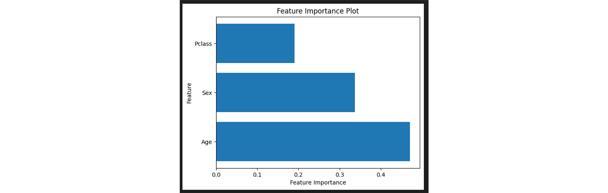
To get more information about the individual features, we can output the Feature Importance:

 1
 2
 3
 4
 5
 6
 7
 8
 9
10
11

# Extract the feature importances
importances = clf.feature_importances_

# Plot a bar chart to visualize the feature importances
features = X_train.columns
indices = np.argsort(importances)[::-1]
plt.barh(features[indices], importances[indices])
plt.xlabel('Feature Importance')
plt.ylabel('Feature')
plt.title('Feature Importance Plot')
plt.show()

Conclusion

As shown, a Random Forest Classifier can be trained quickly and easily with relatively little effort and with relatively good results. Of course, there are many more ways to improve the prediction accuracy. Besides hyperparameter tuning, feature engineering, additional features and better or cleaned data, the prediction accuracy could certainly be significantly improved.

As you can see, the ability to analyze is an aspect that makes the Random Forests algorithm and decision trees in general so interesting. Being able to understand and analyze every decision of the decision tree exactly is a huge advantage when creating, training and further developing models.

Of course, besides Random Forest, there are other algorithms to solve classification problems like this. Examples would be Boosted Trees, Support Vector Machines, Logistic Regression, Neural Networks etc.. Each of these algorithms has its own advantages and disadvantages, depending on the data basis, application and objective, but these will be topics for future articles. Stay tuned! 🚀

This techup has been translated automatically by Gemini