Machine Learning with Tensorflow

My last TechUp was about the basics of deep learning. We got to know key concepts and terms. Today we’re go one step further and deal with the topic of TensorFlow. TensorFlow is an “end-to-end open source machine learning platform”. It was originally developed by Google, but is now available under an open source license. The focus is primarily on speech recognition and image processing. This is possible thanks to neural networks.

Knowing the basics of Python, machine learning concepts and matrix calculation are definitely recommended for using TensorFlow.

Setup 💻

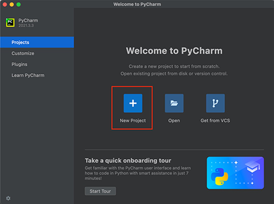
An installation of Python is required for the basic setup. You can check whether you are using the correct version with the python3 --version command. A version between 3.7 and 3.10. is recommended. You also need the Python package manager (pip) in version >19.0 ( or >20.3 for macOS). In addition, you’ll need an IDE, which is where JetBrains’ PyCharm comes in handy. You can download it here.

You can then create a new project using PyCharm. The only thing to note here is that you have to specify the desired name and select the correct Python version.

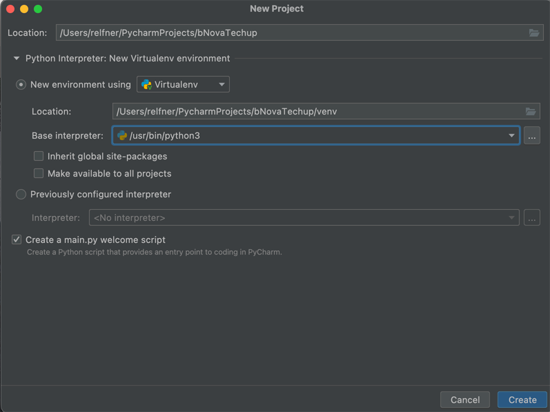
Once the project has been set up, you need a file called requirements.txt, in which you specify which versions of the specified packages should be used. Within the Tensorflow Installation Guide, this is described as follows:

1
2
3
4
5
6

tensorflow==2.7.0
tensorflow-datasets==4.4.0
Pillow==8.4.0
pandas==1.3.4
numpy==1.21.4
scipy==1.7.3

The IDE will then show you a message for you to install the requirements. If you do it that way, you’ll get this display:

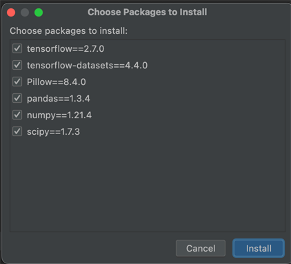
Once the installation is complete, you can open the Python Console.

Unfortunately, in our case, there were issues with the M1 processor. For this reason we have chosen a different variant, which is to use TensorFlow locally. First of all, an installation of Miniforge was necessary. With that, it’s possible to install Python packages, which were compiled natively for the Apple silicon chip.

1

brew install miniforge

After the installation, you can deactivate the standard environment.

1

conda config --set auto_activate_base false

For our example, we created a virtual environment with Python version 3.8. Once created, it still needs to be activated.

1
2

conda create --name mlp python=3.8
conda activate mlp

Now you can start installing all the necessary dependencies. This includes all TensorFlow dependencies first, before you install further requirements via pip for TensorFlow.

1
2
3
4
5
6
7

conda install -c apple tensorflow-deps
pip install tensorflow-macos
conda install -c conda-forge -y pandas jupyter
pip install tensorflow_datasets
pip install Pillow
pip install numpy
python -m pip install -U matplotlib

You should then be at the same level as when installing within the IDE. Assuming there were no errors. In our case, we then used the console within Jupyter using jupyter notebook.

Now we must do the following steps:

import tensorflow as tf

Here it can happen that you get some warnings, if you have a GPU setup on your machine. However, this is not relevant for our case.

To check whether tensorflow is in the correct version, you can output the version in the console: print(tf.__version__).

These are all the necessary imports:

 1
 2
 3
 4
 5
 6
 7
 8
 9
10
11
12
13

import tensorflow as tf
import tensorflow_datasets as tfds
from PIL import Image
import numpy as np
import urllib3 
import pandas as pd
import matplotlib.pyplot as plt

print(tf.__version__)
print(tfds.__version__)
print(Image.__version__)
print(np.__version__)
print(pd.__version__)

Hands-on 🙏

Example MNIST database

Now we want to use the MNIST database as a first example, which is used as a Hello World program compared to other programming languages. The goal is to use a machine learning model that recognizes handwritten digits.

To do this, we first create a new Python file and import all the necessary libraries. The remaining requirements have already been loaded via the requirements file. With the import of os, it’s possible to set environment variables, as can be seen from the log level.

As a third step, a main block is created into which we load the training data from the MNIST database, including some information. The training data is defined as mnist_train and the loaded information is stored in the variable info. In addition, the training data must be loaded.

1
2
3
4
5
6
7
8
9

import tensorflow as tf
import tensorflow_datasets as tfds
import os

os.environ['TF_CPP_MIN_LOG_LEVEL'] = '2'

if __name__ == '__main__':
    mnist_train, info = tfds.load('mnist', split='train', as_supervised=True, with_info=True)
    mnist_test = tfds.load('mnist', split='test', as_supervised=True)   

As soon as you run this file, you’ll get the following output in the console.

1
2
3
4
5

Downloading and preparing dataset 11.06 MiB (download: 11.06 MiB, generated: 21.00 MiB, total: 32.06 MiB) to /Users/relfner/tensorflow_datasets/mnist/3.0.1...

Dl Completed...: 100% 4/4 [00:03<00:00, 1.01 file/s]

Dataset mnist downloaded and prepared to /Users/relfner/tensorflow_datasets/mnist/3.0.1. Subsequent calls will reuse this data.

Now that you have defined the variable info, you can simply print it in the console by calling it up. You can now also visualize your training data. In the example of the MNIST database, these are images of handwritten numbers. To do this, use this command:

1

tfds.show_examples(mnist_train, info)

Once you have executed this command, you will see the following image:

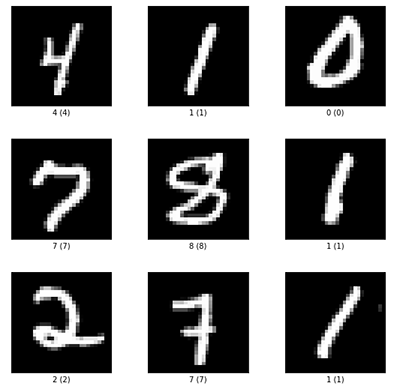
Now you need a method that brings the data into the desired form. In our case, the images are represented as pixel numbers from 1 to 255. However, if you use machine learning, the data should ideally be between 0 and 1. A map function containing a lambda is now used for this. The image that is to be normalized and the label are passed as parameters. However, the label should remain the same. In order to gain performance, the data is loaded into the cache. In the case of the database, this does not have a major impact on the rest of the system.

If the dataset is the training data, the numbers should be randomised. The data set can then be returned.

1
2
3
4
5
6

def wrangle_data(dataset, split):
    wrangled = dataset.map(lambda img, lbl: (tf.cast(img, tf.float32) / 255.0, lbl))
    wrangled = wrangled.cache()
    if split == 'train':
        wrangled = wrangled.shuffle(60000)
    return wrangled.batch(64).prefetch(tf.data.AUTOTUNE)

This method can be defined before the main block. It can then be called within the main block and reassigned to the variable.

1
2

train_data = wrangle_data(mnist_train, 'train')
test_data = wrangle_data(mnist_test, 'test')

Now it’s still necessary to create a model. A new function named create_model is created for this. This is where Keras is used for the first time. The first layer has a “shape” of 28 pixels x 28 pixels x 1 color channel. With the function Flatten(), the layer becomes a single layer. During that process, the content of the shape is multiplied (28x28x1 = 784). With the function Dense(), the model is “fed”, it learns the the differences and finds out how to classify the data.

Finally, another function is called, which is created in the next step.

1
2
3
4
5
6
7
8

def create_model():
    new_model = tf.keras.Sequential([
        tf.keras.layers.InputLayer((28, 28, 1)),
        tf.keras.layers.Flatten(),
        tf.keras.layers.Dense(64, activation='relu'),
        tf.keras.layers.Dense(10, activation='softmax')
    ])
    return compile_model(new_model)

This function must be called inside the main block:

1

model = create_model()

Now another function is necessary for compiling the model, which is defined as an input parameter. The function compile() defines the optimizer, the loss function and the metrics for further information.

1
2
3
4

def compile_model(new_model):
    new_model.compile(optimizer='adam', loss='sparse_categorical_crossentropy', metrics=['accuracy'])
    print(new_model.summary())
    return new_model

As soon as this function is finished, you can run your program again. You will receive some information as an output. You can see how many parameters are processed per layer and how correctness improves per pass.

 1
 2
 3
 4
 5
 6
 7
 8
 9
10
11
12
13
14
15
16
17
18
19
20
21
22
23
24
25
26

Model: "sequential"
_________________________________________________________________
 Layer (type)                Output Shape              Param # 
=================================================================
 flatten (Flatten)           (None, 784)               0         
                                                                 
 dense (Dense)               (None, 64)                50240     
                                                                 
 dense_1 (Dense)             (None, 10)                650       
                                                                 
=================================================================
Total params: 50,890
Trainable params: 50,890
Non-trainable params: 0
_________________________________________________________________
None
Epoch 1/5
938/938 [==============================] - 7s 5ms/step - loss: 0.3554 - accuracy: 0.9024
Epoch 2/5
938/938 [==============================] - 4s 5ms/step - loss: 0.1787 - accuracy: 0.9489
Epoch 3/5
938/938 [==============================] - 4s 4ms/step - loss: 0.1326 - accuracy: 0.9621
Epoch 4/5
938/938 [==============================] - 4s 5ms/step - loss: 0.1050 - accuracy: 0.9691
Epoch 5/5
938/938 [==============================] - 4s 5ms/step - loss: 0.0875 - accuracy: 0.9743

To check how well the model has been trained, you can use the test data from the first step and use the evaluate() function. You can see the accuracy that has been achieved using data that the model has not yet known.

1
2
3
4

model.evaluate(test_data)

157/157 [==============================] - 1s 5ms/step - loss: 0.0971 - accuracy: 0.9702
[0.09706369042396545, 0.9702000617980957]

If you now want to save your work, you can do so with model.save('mnist.h5'). Within your project, you will now find that file.

Example online data

If you want to use a model with data from the internet, check out the Machine Learning Repository. The most used data set is the Iris Dataset.

To do this, you first need a function that loads the relevant data from the Internet. For this, you need the corresponding Url and the desired storage location must be defined.

1
2
3
4
5
6
7

def loadData():
    data_source_url = 'https://archive.ics.uci.edu/ml/machine-learning-databases/iris/iris.data'
    cache_dir = '.'
    cache_subdir = 'data'
    data_file = tf.keras.utils.get_file('iris.data', data_source_url, cache_dir=cache_dir, cache_subdir=cache_subdir)

    return data_file

This function can now be called within a main block so that the data is loaded.

1
2

if __name__ == "__main__":
    iris_filepath = loadData()

As soon as you run the file for the first time, the data is available to you. In any case, it’s recommended to look at the data for the model first, to check whether it corresponds to the desired format or needs to be adjusted.

1
2
3
4
5
6

head -5 data/iris.data

5.1,3.5,1.4,0.2,Iris-setosa
4.9,3.0,1.4,0.2,Iris-setosa
4.7,3.2,1.3,0.2,Iris-setosa
4.6,3.1,1.5,0.2,Iris-setosa

In this case we are missing the names of the columns. Therefore, you’ll have to add them so that the data can be assigned. To do this, you first create an array with the appropriate name. Instead of names, numbers should be used so that the model can handle them better. For this, we create a map which assigns the corresponding types to a number.

1
2
3
4
5
6
7

iris_columns = ['sepal_length', 'sepal_width', 'petal_length', 'petal_width', 'species']
label_map= {'Iris-setosa': 0, 'Iris-versicolor': 1, 'Iris-virginica': 2}

def parseData(iris_path):
    iris_df = pd.read_csv(iris_path, names=iris_columns)
    iris_df['species'].replace(label_map, inplace=True)
    return iris_df

This function can now also be called within the main block iris_data = parse_iris_data(iris_filepath). To check your result, you can compare the number of “species”. There should be 50 of each species.

1
2
3
4
5
6

iris_data['species'].value_counts()

0    50
1    50
2    50
Name: species, dtype: int64

Finally, the data needs to be loaded into a TensorFlow dataset. You now create another function for this. To define this set, you must first determine the features. These correspond to the column names. In this example, iris_columsn can be used directly. The labels must then also be read from the dataframe.

1
2
3

iris_columns[:4] --> ['sepal_length', 'sepal_width', 'petal_length', 'petal_width']

iris_columns[-1] --> species

This function must also be called in the main block.

1
2
3
4
5

def createDataset(iris_dataframe):
    features = iris_dataframe[iris_columns[:4]]
    labels = iris_dataframe[iris_columns[-1]]
    iris_dataset = tf.data.Dataset.from_tensor_slices((features, labels))
    return iris_dataset

The end result would now look like this:

 1
 2
 3
 4
 5
 6
 7
 8
 9
10
11
12
13
14
15
16
17
18
19
20
21
22
23
24
25
26
27
28
29
30
31
32
33
34

import os

os.environ['TF_CPP_MIN_LOG_LEVEL'] = '2'

def loadData():
    data_source_url = 'https://archive.ics.uci.edu/ml/machine-learning-databases/iris/iris.data'
    cache_dir = '.'
    cache_subdir = 'data'
    data_file = tf.keras.utils.get_file('iris.data', data_source_url, cache_dir=cache_dir, cache_subdir=cache_subdir)

    return data_file


iris_columns = ['sepal_length', 'sepal_width', 'petal_length', 'petal_width', 'species']
label_map = {'Iris-setosa': 0, 'Iris-versicolor': 1, 'Iris-virginica': 2}


def parseData(iris_path):
    iris_df = pd.read_csv(iris_path, names=iris_columns)
    iris_df['species'].replace(label_map, inplace=True)
    return iris_df


def createDataset(iris_dataframe):
    features = iris_dataframe[iris_columns[:4]]
    labels = iris_dataframe[iris_columns[-1]]
    iris_dataset = tf.data.Dataset.from_tensor_slices((features, labels))
    return iris_dataset

if __name__ == "__main__":
    iris_filepath = loadData()

iris_data = parseData(iris_filepath);
iris_ds = createDataset(iris_data)

Once this code is executed, the appropriate data is downloaded, prepared, and loaded into the dateset.

Conclusion ✨

In this TechUp we were able to go one step further, since we already laid the foundations for the topic last time. That’s why we’ve dedicated ourselves to the practical part today, using the most well-known database in the field of machine learning. Furthermore, we were able to show how easy it is to create an ML model with the help of TensorFlow and how to train and test it directly. We were also able to go one step further and use data from the Internet. This means that we are now able to use existing data, since you can save a lot of time here if you don’t have to collect your own data. But at this point it’s important to say that these are very simple basics in the area of TensorFlow. So there are many more exciting topics in this area that we will look at.

Stay tuned! 🚀