Figure: PyTorch, the PyTorch logo and any related marks are trademarks of The Linux Foundation.

With the help of Machine Learning algorithms, a lot of interesting and valuable information can be extracted from large data sets. Depending on the use case, different algorithms are suitable for different scenarios. In previous TechUps, Stefan has already explained the basics of neural networks and we have seen how the Random Forest algorithm can be used to predict the survival probability of passengers on the Titanic ship. In this TechUp, we want to look at another technique that helps us detect patterns in data: Anomaly Detection.

What is Anomaly Detection?

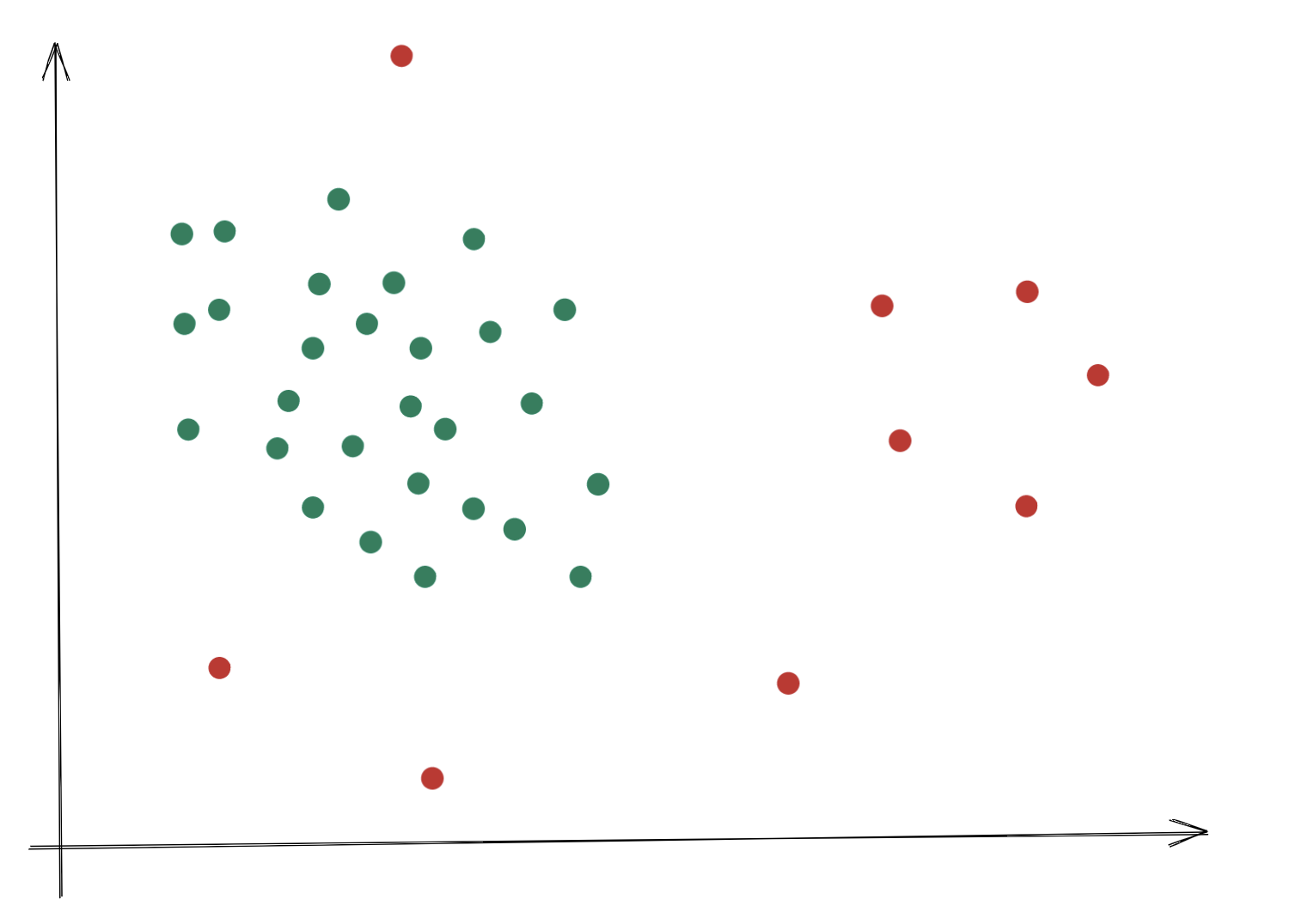
Anomaly Detection is a method we use to find out whether a certain event related to a dataset conforms to the norm or not. There are many use cases that can illustrate this.

Take, for example, the sensor system of a machine that provides data points about vibrations at various measuring points. If we record this data over a longer period of time, we can see patterns that show what kind of vibrations the machine normally exhibits. As soon as data points are measured that deviate from these patterns, we can assume that the machine is no longer in normal condition. This can be an indication that the machine is defective and needs to be repaired.

Other use cases exist in many areas:

• Cybersecurity (e.g. detection of anomalies in network traffic).
• Fraud detection (e.g. credit card fraud or insurance fraud)
• Healthcare (e.g. rare disease detection)
• Road traffic (e.g. detection of accidents)

How does Anomaly Detection work?

As we have seen, there are many use cases where Anomaly Detection can be used. If we want to use Machine Learning algorithms to detect anomalies, there are two different approaches that we will look at below.

However, before we think about training models, we should first think about the data basis. First of all, in order to be able to detect anomalies, data is needed that represents the normal state. Depending on the algorithm, classified data may also be needed that deviates sufficiently from the norm to be classified as an anomaly in the first place. Especially in anomaly detection, the quality of the data basis is crucial. Consider fraud detection, for example: we can assume that the majority of data points are not fraudulent. If the few fraudulent data points are not sufficiently representative or are misclassified, our algorithm may make incorrect predictions. In this case, this can lead to over- or under-classification, which can have severe consequences depending on the field of application.

Now, once the quality of the data basis is assured, we can think about the algorithms. Here we distinguish between two different approaches: Supervised Learning and Unsupervised Learning. If we want to use a Supervised Learning algorithm, our data set must be classified, which means that each data point must be classified as either a normal state or an anomaly. Depending on the use case, it can be difficult to generate such data.

If we look at the example of a machine’s sensors, we would expect few to no anomalies to occur under normal circumstances. However, if we want to take a supervised approach, we would either need to collect data over relatively long periods of time or purposefully damage or disrupt the machine to generate anomaly data points. Classifying the sensor data correctly is also not necessarily easy. In such cases, an Unsupervised Learning Algorithm is better suited, which does not require previously classified data, but uses pattern recognition to detect the anomalies itself.

Example: Anomaly detection based on credit card fraud

To illustrate the two approaches, let’s look at a data set on credit card fraud as an example. The data includes a total of almost 284,000 credit card transactions over two days in September 2013, of which 492 were classified as fraudulent. The dataset can be downloaded from Kaggle.

In total, we have 30 numerical features, 28 of which are the result of a Principal Component Analysis (PCA) transformation of the original data. The other two characteristics are the time and the amount of the transaction. Due to anonymisation measures, no further information on the individual features is known.

Since we have classified data, we can use a supervised learning approach. Here we will use the Random Forest Algorithm, which we already learned about in my TechUp on Decision Trees.

As another approach, we will also introduce Autoencoder after this example to illustrate an Unsupervised Learning algorithm.

Anomaly Detection with Random Forest

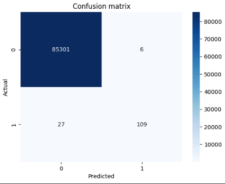
The Random Forest algorithm can be used to train a model that can classify individual data points based on their features. To train the model, we need classified data, which we find in our data set. We will now train the model and then compare the predictions of the model with the actual classifications. 🤓

 1
 2
 3
 4
 5
 6
 7
 8
 9
10
11
12
13
14
15
16
17
18
19
20
21
22
23
24
25
26
27
28
29
30
31
32
33
34

import pandas as pd
import numpy as np
from sklearn.model_selection import train_test_split
from sklearn.ensemble import RandomForestClassifier
from sklearn.metrics import classification_report, confusion_matrix
import matplotlib.pyplot as plt
import seaborn as sns


# Loading the Credit Card Fraud Detection dataset from Kaggle
df = pd.read_csv('creditcard.csv')

# Splitting the dataset into training and testing sets
X_train, X_test, y_train, y_test = train_test_split(df.drop('Class', axis=1), df['Class'], test_size=0.3, random_state=42)

# Creating a Random Forest classifier object
rfc = RandomForestClassifier(n_estimators=100, random_state=42)
# Fitting the Random Forest classifier to the training data
rfc.fit(X_train, y_train)

# Making predictions on the testing data
y_pred = rfc.predict(X_test)

# Printing the confusion matrix and classification report
print(confusion_matrix(y_test, y_pred))
print(classification_report(y_test, y_pred))

# Plotting the confusion matrix
cm = confusion_matrix(y_test, y_pred)
sns.heatmap(cm, annot=True, fmt='g', cmap='Blues')
plt.xlabel('Predicted')
plt.ylabel('Actual')
plt.title('Confusion matrix')
plt.show()

The results are quite worth seeing, despite the little effort involved:

Anomaly Detection with Autoencoders

Autoencoders are a special type or architecture of neural networks that are designed to compress data. The idea behind autoencoders is best explained with the help of an illustration:

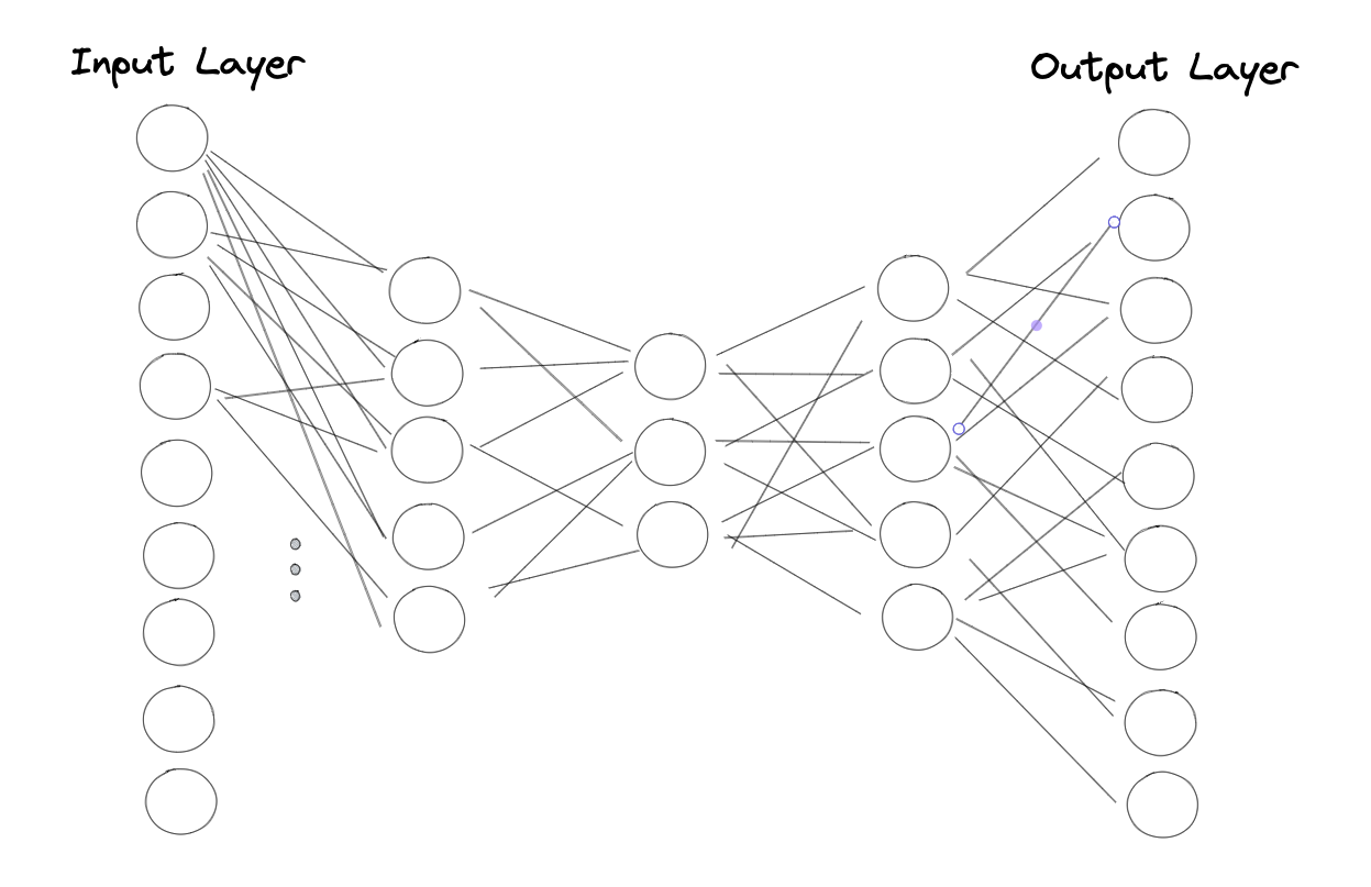
We see a neural network with one input, one output and three hidden layers. All layers are fully interconnected, that is, all neurons are connected to all neurons of the previous and subsequent layers. As you can see, the number of neurons decreases from layer to layer and the network is mirrored in the middle.

What is special about autoencoders is the way they are trained. The network is trained to provide the same output as input. If we take our dataset as an example, we would expect the same values in the output for every feature in every data point. The tapering of the layers means that the network has to compress the input data to the most important features or information in order to reproduce them in the output.

The trained model has now learned the structure of the training data and can classify new data points based on this structure. If one now wants to classify a new data point, it is pushed through the network and the output of the network is compared with the input. The greater the difference between input and output, the more the data point deviates from the structure of the training data and the more likely it is to be an anomaly. Cool, isn’t it? 😎

Below we train an autoencoder with PyTorch and use it to classify new data points.

 1
 2
 3
 4
 5
 6
 7
 8
 9
10
11
12
13
14
15
16
17
18
19
20
21
22
23
24
25
26
27
28
29
30
31
32
33
34
35
36
37
38
39
40
41
42
43
44
45
46
47
48
49
50
51
52
53
54
55
56
57
58
59
60
61
62
63
64
65
66
67

import torch
import torch.nn as nn
import torch.optim as optim
import numpy as np
import pandas as pd
from sklearn.preprocessing import StandardScaler
from sklearn.model_selection import train_test_split

data = pd.read_csv("creditcard.csv")

scaler = Normalizer()
data.iloc[:, 1:29] = scaler.fit_transform(data.iloc[:, 1:29])

# Scale the data
scaler = MinMaxScaler()
data.iloc[:, 1:29] = scaler.fit_transform(data.iloc[:, 1:29])

# Separate the non-fraud cases
non_fraud_data = data[data.Class == 0].iloc[:, 1:29].values
fraud_data = data[data.Class == 1].iloc[:, 1:29].values


# Define the autoencoder architecture
class Autoencoder(nn.Module):
    def __init__(self):
        super(Autoencoder, self).__init__()
        self.encoder = nn.Sequential(
            nn.Linear(28, 16),
            nn.ELU(True),
            nn.Linear(16, 8),
            nn.ELU(True),
            nn.Linear(8, 4),
            nn.ELU(True))
        self.decoder = nn.Sequential(
            nn.Linear(4, 8),
            nn.ELU(True),
            nn.Linear(8, 16),
            nn.ELU(True),
            nn.Linear(16, 28),
            nn.ELU(True))

    def forward(self, x):
        x = self.encoder(x)
        x = self.decoder(x)
        return x

# Initialize the autoencoder
autoencoder = Autoencoder()

# Define the loss function and optimizer
criterion = nn.MSELoss()
optimizer = optim.Adam(autoencoder.parameters(), lr=0.01)

# Train the autoencoder
num_epochs = 20
batch_size = 256
for epoch in range(num_epochs):
    np.random.shuffle(non_fraud_data)
    for i in range(0, len(non_fraud_data), batch_size):
        batch = non_fraud_data[i:i+batch_size]
        batch = torch.FloatTensor(batch)
        optimizer.zero_degree()
        outputs = autoencoder(batch)
        loss = criterion(outputs, batch)
        loss.backward()
        optimizer.step()
    print('Epoch [{}/{}], Loss: {:.4f}'.format(epoch+1, num_epochs, loss.item()))

We can now evaluate the trained model with the pre-classified data points. To do this, we compare the differences between the input and output of the autoencoder (loss) of a subset of the non-fraud data points with those of the fraud data points. The greater the difference between the two data sets, the better the model is at detecting anomalies.

 1
 2
 3
 4
 5
 6
 7
 8
 9
10
11
12
13
14
15
16
17
18
19
20
21

non_fraud_loss = []
for i in range(0, 500):
x = torch.FloatTensor(non_fraud_data[i])
output = autoencoder(x)
loss = criterion(output, x)
non_fraud_loss.append(loss.item())

fraud_loss = []
for i in range(0, len(fraud_data)):
x = torch.FloatTensor(fraud_data[i])
output = autoencoder(x)
loss = criterion(output, x)
fraud_loss.append(loss.item())

bins = np.linspace(0, 0.04, 200)
plt.hist(non_fraud_loss, bins, alpha=0.5, color='green', label='Non-Fraud')
plt.hist(fraud_loss, bins, alpha=0.5, color='red', label='Fraud')
plt.xlabel('Loss')
plt.ylabel('Count')
plt.legend(loc='upper right')
plt.show()

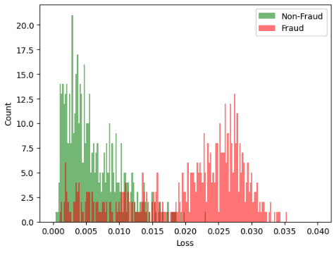
As you can see in the figure, the loss values of the fraud data points differ significantly from those of the non-fraud data points. We can now define a threshold value from which a data point is classified as an anomaly.

Of course, our classification is not optimal, as can be seen from the overlap of the two histograms. Whether autoencoders are the right tool for detecting anomalies depends strongly on the data and must always be evaluated individually.

Conclusion

I hope I could give you an interesting insight into the field of anomaly detection with this TechUp. There are many areas where you can gain valuable information by detecting data points that deviate from the (supposed) norm. Stay tuned! 🙌

Why don’t you read Stefan’s TechUp on the basics of neural networks! 🚀

This TechUp was translated by our automatic Markdown Translator. 🙌